
Excel Pivot Table
How to Apply Conditional Formatting in Excel Pivot Table
Learn how to apply conditional formatting in Excel Pivot Tables using the formatting icon or by creating a new conditional rule.
Read article

24 articles tagged with “Excel Conditional Formatting”
Learn how to apply conditional formatting in Excel Pivot Tables using the formatting icon or by creating a new conditional rule.

Learn how to highlight entire row in Excel with conditional formatting using cell values, numeric criteria, logical functions or dropdowns.

Learn how to show data bars with percentage in Excel using conditional formatting, the REPT function, and options for negative values.

Learn how to apply conditional formatting to blank cells in Excel using the built-in “Blanks” option, ISBLANK, OR, LEN functions & formulas.
Learn how to apply Excel conditional formatting based on another cell range using operators, text rules, AND/OR logic, and VBA.
Learn how to copy conditional formatting to another sheet in Excel using Format Painter, Paste Special, rule manager, or VBA automation.
Learn how to use conditional formatting in Excel to highlight overdue dates with formulas, COUNTIF, partial matches and dynamic named ranges.

Learn how to apply conditional formatting based on anothr cell with multiple values using OR, COUNTIF, partial matches, and named range

Learn how to highlight a cell in Excel if its value is greater than another cell using conditional formatting, formulas, and built-in rules.
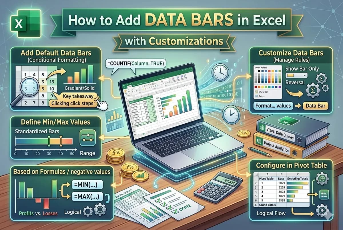
Learn how to add data bars in Excel using conditional formatting, customize them, and apply them to pivot tables and formulas.
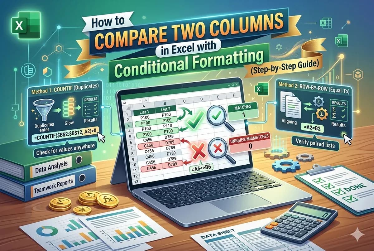
Learn how to use conditional formatting in Excel to compare two columns and highlight matching or unique values easily.
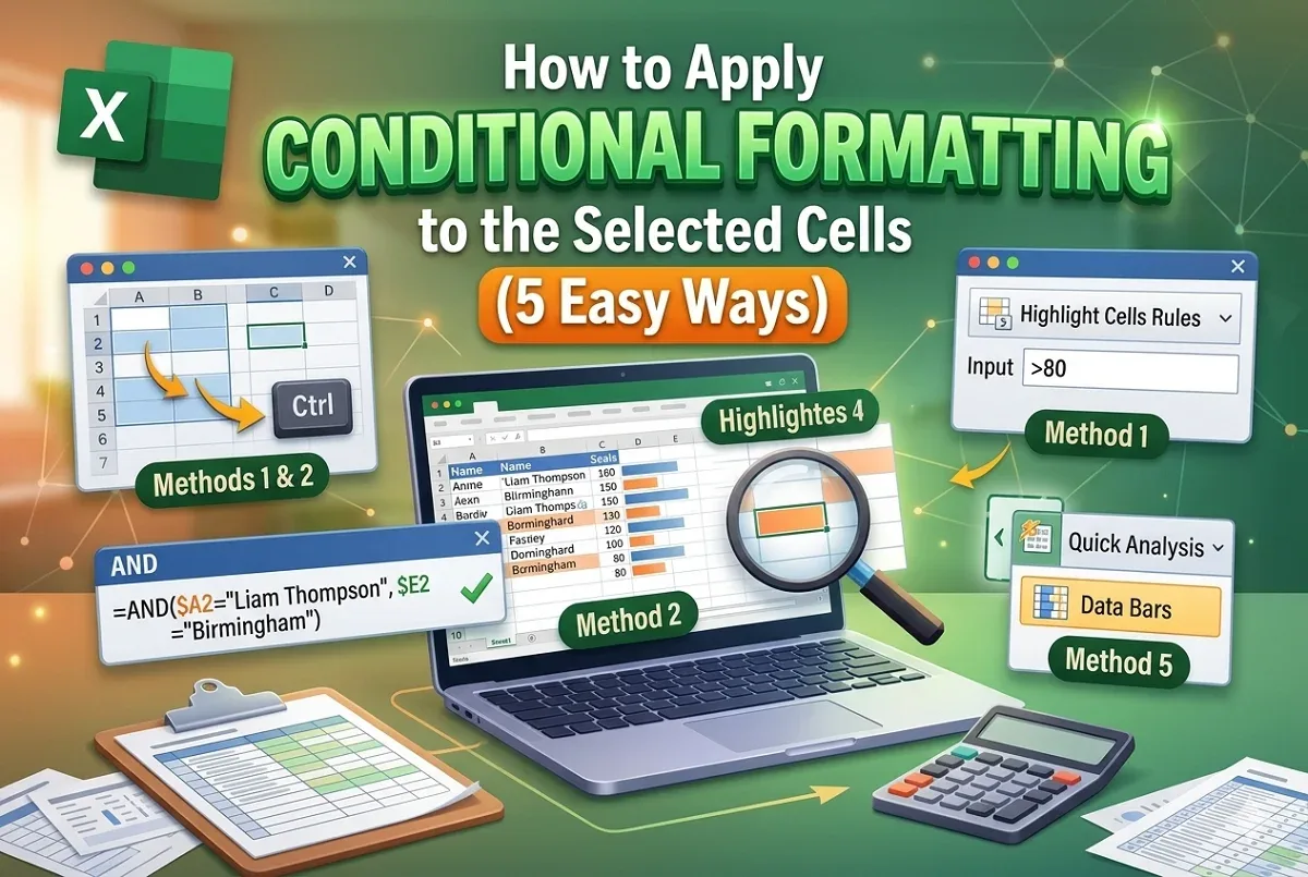
This article shows 5 ways to apply conditional formatting to selected non-adjacent cells, two columns, with formulas, & data bars option